Density and public transportation

Sufficient population and job density are important for a public transportation system. Therefore plotting densities and public transportation systems on the same map can reveal opportuntities to build more public transportation lines (where density is high, but there are no existing lines) and to build more housing/jobs (where public transportation lines exist, but densities are low).

Let’s create a map of population density. In the United States, we can get this geo-tagged population data from the United States Census Bureau. dpd.modeling has a class Zones to store this data and a method to automatically pull this data from the United States Census Bureau.

First, we’ll define the state that we are interested in mapping. States seems to be the best level to get data for. If we get data by county, there are lots of requests so it takes too long. However, data for the whole country is unnecessary.

import us
from ipywidgets import Select
from IPython.display import display

YEAR = "2017"

state = Select(
    options=list(map(lambda x: x.name, us.STATES)),
    description="State",
    value="California",
)
display(state)

Now we can get the census data for California. The government assigns a number to each state so California is 06. B01003_001E is the population in each census tract. This is renamed to Total Population. Also, ALAND is the land area of the zone. We use these two values to compute a density as population per area. Also, we simplify the geometry column to speed up any geometric computations.

from dpd.modeling import Zones

zones = Zones.from_uscensus(str(us.states.lookup(state.value).fips), YEAR)

zones["geometry"] = zones["geometry"].apply(lambda x: x.simplify(0.001))

zones.head(1)

/home/docs/checkouts/readthedocs.org/user_builds/dpd/envs/latest/lib/python3.9/site-packages/dpd/modeling/zones.py:58: FutureWarning: Downcasting object dtype arrays on .fillna, .ffill, .bfill is deprecated and will change in a future version. Call result.infer_objects(copy=False) instead. To opt-in to the future behavior, set `pd.set_option('future.no_silent_downcasting', True)`
  zones["Worker Population"] = zones["Worker Population"].fillna(0).apply(int)

	Name	Total Population	Worker Population	state	county	tract	STATEFP	COUNTYFP	TRACTCE	NAME_y	...	FUNCSTAT	ALAND	AWATER	INTPTLAT	INTPTLON	geometry	Total Population + Worker Population	Total Population Density	Worker Population Density	Total Population + Worker Population Density
GEOID
6037503502	Census Tract 5035.02, Los Angeles County, Cali...	4359	0	06	037	503502	06	037	503502	5035.02	...	S	1244436	0	+33.9320286	-118.0031960	POLYGON ((-118.01180 33.92688, -118.01169 33.9...	4359	0.003503	0.0	0.003503

1 rows × 22 columns

Here we can plot the population density of California.

zones.explore(
    column="Total Population + Worker Population Density", scheme="JenksCaspall", k=20
)

Make this Notebook Trusted to load map: File -> Trust Notebook

For the rest of the notebook, we will focus on Los Angeles County. We can query OpenStreetMap for the geometric data that represents Los Angeles County and then combine it with our Zones to reduce the amount of data to process

from shapely.geometry import Polygon
from shapely.ops import linemerge

from dpd.osm import OSM

relation = 396479  # Los Angeles County
osm = OSM()
osm.download_relation(relation)
ways = [
    osm.ways[member["ref"]].geo
    for member in osm.relations[relation]["members"]
    if member["type"] == "way"
]
ways

ways_merged = linemerge(ways)
longest_length = 0
for way in ways_merged.geoms:
    if way.length > longest_length:
        longest_length = way.length
        longest_way = way
los_angeles_county = Polygon(longest_way)

los_angeles_county

zones.geometry.within(los_angeles_county).value_counts()

False    5770
True     2287
Name: count, dtype: int64

zones = zones[zones.geometry.within(los_angeles_county)]

Now we can use h3fy to recompute our population density into hexigons. This normalizes the geometries so they can be used for calculations later on.

from tobler.util import h3fy
from tobler.area_weighted import area_interpolate

zones.to_crs(epsg=4087, inplace=True)
h3_zones = h3fy(zones, buffer=True)

interpolated = area_interpolate(
    source_df=zones,
    target_df=h3_zones,
    intensive_variables=["Total Population", "Worker Population", "ALAND"],
)
zones_interpolated = Zones(interpolated)
zones_interpolated["Total Population Density"] = (
    zones_interpolated["Total Population"] / zones_interpolated["ALAND"]
)
zones_interpolated["Worker Population Density"] = (
    zones_interpolated["Worker Population"] / zones_interpolated["ALAND"]
)
zones_interpolated["Total Population + Worker Population"] = (
    zones_interpolated["Total Population"] + zones_interpolated["Worker Population"]
)
zones_interpolated["Total Population + Worker Population Density"] = (
    zones_interpolated["Total Population + Worker Population"]
    / zones_interpolated["ALAND"]
)
zones_interpolated.head(1)

/home/docs/checkouts/readthedocs.org/user_builds/dpd/envs/latest/lib/python3.9/site-packages/pyproj/crs/crs.py:1293: UserWarning: You will likely lose important projection information when converting to a PROJ string from another format. See: https://proj.org/faq.html#what-is-the-best-format-for-describing-coordinate-reference-systems
  proj = self._crs.to_proj4(version=version)

	Total Population	Worker Population	ALAND	geometry	Total Population Density	Worker Population Density	Total Population + Worker Population	Total Population + Worker Population Density
hex_id
8629a1227ffffff	5610.0	0.0	615828928.0	POLYGON ((-13225816.667 3864719.878, -13222265...	0.000009	0.0	5610.0	0.000009

And we can plot the hexigons.

zones_interpolated.explore(
    column="Total Population + Worker Population Density", scheme="JenksCaspall", k=20
)

Make this Notebook Trusted to load map: File -> Trust Notebook

These hexigons are pretty big. Let’s recompute them to be smaller and plot with lonboard. Lonboard is great for plotting lots of data quickly.

import numpy
from lonboard import Map, SolidPolygonLayer
from mapclassify import JenksCaspall
from palettable.matplotlib import Viridis_20

h3_zones = h3fy(zones, resolution=8, buffer=True)

interpolated = area_interpolate(
    source_df=zones,
    target_df=h3_zones,
    intensive_variables=["Total Population", "Worker Population", "ALAND"],
)
zones_interpolated = Zones(interpolated)
zones_interpolated["Total Population Density"] = (
    zones_interpolated["Total Population"] / zones_interpolated["ALAND"]
)
zones_interpolated["Worker Population Density"] = (
    zones_interpolated["Worker Population"] / zones_interpolated["ALAND"]
)
zones_interpolated["Total Population + Worker Population"] = (
    zones_interpolated["Total Population"] + zones_interpolated["Worker Population"]
)
zones_interpolated["Total Population + Worker Population Density"] = (
    zones_interpolated["Total Population + Worker Population"]
    / zones_interpolated["ALAND"]
)

layer = SolidPolygonLayer.from_geopandas(zones_interpolated, opacity=0.1)
jc = JenksCaspall(
    zones_interpolated["Total Population + Worker Population Density"].fillna(0), k=10
)
colors = []
for color in jc.yb:
    colors.append(Viridis_20.colors[color])
layer.get_fill_color = numpy.uint8(colors)

Map(layers=[layer])

/home/docs/checkouts/readthedocs.org/user_builds/dpd/envs/latest/lib/python3.9/site-packages/pyproj/crs/crs.py:1293: UserWarning: You will likely lose important projection information when converting to a PROJ string from another format. See: https://proj.org/faq.html#what-is-the-best-format-for-describing-coordinate-reference-systems
  proj = self._crs.to_proj4(version=version)
/home/docs/checkouts/readthedocs.org/user_builds/dpd/envs/latest/lib/python3.9/site-packages/lonboard/_geoarrow/ops/reproject.py:97: UserWarning: Input being reprojected to EPSG:4326 CRS
  warnings.warn("Input being reprojected to EPSG:4326 CRS")

Now, it would be helpful to do the same exercise with job densiites. However, the US Census Bureau does not provide this information (“Worker Population”: “B08604_001E”) at the tract level like they do for population. This leaves us with two options which both require large downloads.

1. We can download zip code worker populations.

2. Or we can download LODES data which includes origin-destination information.

We’ll take a look at option 2 below. The LODES data is divided into three files: residential data, work data, and origin-destination data. There is also a cross-walk file that includes a translation from LODES GEOIDs to census tracts.

from dpd.modeling import TripDataFrame

"""
od = TripDataFrame.from_lodes(us.states.lookup(state.value).abbr.lower(), YEAR)

od.head()"""

'\nod = TripDataFrame.from_lodes(us.states.lookup(state.value).abbr.lower(), YEAR)\n\nod.head()'

We can then combine the LODES data with our original output DataFrame (which includes the geometry) to add a job_density column.

"""zones = Zones(zones).production_attraction_from_lodes(od)
h3_zones = h3fy(zones, resolution=9, buffer=True)

interpolated = area_interpolate(
    source_df=zones,
    target_df=h3_zones,
    intensive_variables=["Total Population", "Worker Population", "ALAND"],
)
zones_interpolated = Zones(interpolated)
zones_interpolated["Total Population Density"] = (
    zones_interpolated["Total Population"] / zones_interpolated["ALAND"]
)
zones_interpolated["Worker Population Density"] = (
    zones_interpolated["Worker Population"] / zones_interpolated["ALAND"]
)
zones_interpolated["Total Population + Worker Population"] = (
    zones_interpolated["Total Population"] + zones_interpolated["Worker Population"]
)
zones_interpolated["Total Population + Worker Population Density"] = (
    zones_interpolated["Total Population + Worker Population"]
    / zones_interpolated["ALAND"]
)

zones_interpolated.head(1)"""

'zones = Zones(zones).production_attraction_from_lodes(od)\nh3_zones = h3fy(zones, resolution=9, buffer=True)\n\ninterpolated = area_interpolate(\n    source_df=zones,\n    target_df=h3_zones,\n    intensive_variables=["Total Population", "Worker Population", "ALAND"],\n)\nzones_interpolated = Zones(interpolated)\nzones_interpolated["Total Population Density"] = (\n    zones_interpolated["Total Population"] / zones_interpolated["ALAND"]\n)\nzones_interpolated["Worker Population Density"] = (\n    zones_interpolated["Worker Population"] / zones_interpolated["ALAND"]\n)\nzones_interpolated["Total Population + Worker Population"] = (\n    zones_interpolated["Total Population"] + zones_interpolated["Worker Population"]\n)\nzones_interpolated["Total Population + Worker Population Density"] = (\n    zones_interpolated["Total Population + Worker Population"]\n    / zones_interpolated["ALAND"]\n)\n\nzones_interpolated.head(1)'

And we can plot the job density like we ploted the population density above.

Los Angeles County Metro is planning to extend the C Line south towards Torrance. One of the design decisions is where to put a station: at the South Bay Galleria or Redondo Beach Transit Center? Let’s look at the population density around these two locations. We can buffer the stop locations with a radius of 1000km and plot along with the density.

from folium import Map
from geopandas import GeoSeries
from shapely.geometry import Point

station_locations = GeoSeries(
    data=[
        Point(-118.35884733230867, 33.86557221753289),
        Point(-118.35253437469025, 33.87283256915632),
    ],
    index=["South Bay Galleria", "Redondo Beach Transit Center"],
    crs="EPSG:4326",
).to_crs(epsg=4087)

folium_map = Map(location=(33.87, -118.35), zoom_start=14)
station_locations.buffer(1000).explore(m=folium_map)
zones.explore(
    column="Total Population + Worker Population Density",
    scheme="JenksCaspall",
    k=20,
    m=folium_map,
)

Make this Notebook Trusted to load map: File -> Trust Notebook

from dpd.modeling import contour_dataframe

folium_map = Map(location=(33.87, -118.35), zoom_start=14)
zones.explore(
    column="Total Population + Worker Population Density",
    scheme="JenksCaspall",
    k=20,
    m=folium_map,
)
for station_location in station_locations:
    contour_dataframe(station_location, crs=station_locations.crs).explore(m=folium_map)
folium_map

Make this Notebook Trusted to load map: File -> Trust Notebook

from dpd.modeling import DistanceDataFrame

distance_dataframe = DistanceDataFrame.from_origins_destinations(
    zones_interpolated.geometry.centroid,
    station_locations.geometry,
    method="distance",
)
distance_dataframe.columns = station_locations.index
distance_dataframe

	South Bay Galleria	Redondo Beach Transit Center
hex_id
8829a0361dfffff	69363.409109	68374.524691
8829a155c5fffff	82542.833883	81526.637414
8829a1452dfffff	100263.005120	99244.302183
8829a11153fffff	53740.397727	53005.196677
8829a1d5edfffff	34757.881037	33717.646049
...	...	...
8829a114a9fffff	73572.135963	73154.349323
8829a1d9e7fffff	63224.048765	62199.279461
8829a1c19dfffff	51978.474660	50914.794962
8829a1445dfffff	91615.971337	90643.419420
8829a15683fffff	73646.957905	72685.234677

8708 rows × 2 columns

from matplotlib import pyplot as plt

fig = plt.figure(figsize=(18, 16))
ax = fig.add_subplot(111)
(distance_dataframe / 1.35).hist(
    weights=zones_interpolated["Total Population + Worker Population"],
    range=(0, 900),
    bins=30,
    cumulative=True,
    sharey=True,
    ax=ax,
)
ax.set_ylabel("Population (cumulative)")
ax.set_xlabel("Time (seconds)")

/tmp/ipykernel_2518/1319192995.py:5: UserWarning: To output multiple subplots, the figure containing the passed axes is being cleared.
  (distance_dataframe / 1.35).hist(

Text(0.5, 0, 'Time (seconds)')

Now we download our public transportation systems so we can plot the lines. Here we can download the Los Angeles Metro Rail network from OpenStreetMap.

from dpd.driving.network import Network

query = """
[out:json][timeout:25];
(
  relation["network"="Metro Rail"];

);
out body;
>;
out skel qt;
"""

network = Network.from_osm_query(query)

100%|██████████| 14/14 [00:33<00:00,  2.36s/it]

And we can plot the network on the original population density map.

from lonboard import Map, ScatterplotLayer

layer = SolidPolygonLayer.from_geopandas(zones_interpolated, opacity=0.1)
jc = JenksCaspall(
    zones_interpolated["Total Population + Worker Population Density"], k=10
)
colors = []
for color in jc.yb:
    colors.append(Viridis_20.colors[color])
layer.get_fill_color = numpy.uint8(colors)
layers = [layer]
for route in network.routes:
    layers.append(
        ScatterplotLayer.from_geopandas(
            network.routes[route].stops, radius_min_pixels=10
        )
    )

Map(layers=layers)

/home/docs/checkouts/readthedocs.org/user_builds/dpd/envs/latest/lib/python3.9/site-packages/lonboard/_geoarrow/ops/reproject.py:97: UserWarning: Input being reprojected to EPSG:4326 CRS
  warnings.warn("Input being reprojected to EPSG:4326 CRS")

import folium

folium_map = folium.Map(location=(34, -118.3), zoom_start=11)
zones.explore(
    m=folium_map,
    column="Total Population + Worker Population Density",
    scheme="JenksCaspall",
    k=20,
)
for route in network.routes:
    network.routes[route].geometry.explore(m=folium_map)

folium_map

Make this Notebook Trusted to load map: File -> Trust Notebook

Now let’s look at accessibility. We will download one metro line and compute the distance to each stop from each zone.

from astropy import units
from dpd.driving import Route

route = Route.from_osm_relation(relation=2351006)

from dpd.modeling import DistanceDataFrame, TripDataFrame

### Here is the "old way" of computing distances before we used hexogons
# points = zones.polygons_to_points()
# distance_dataframe = DistanceDataFrame.from_origins_destinations(
#     points.geometry, stops.geometry, method="distance"
# )

stops = route.stops.to_crs("EPSG:4087")
distance_dataframe = DistanceDataFrame.from_origins_destinations(
    zones_interpolated.geometry.centroid,
    stops.geometry,
    method="distance",
)
distance_dataframe.columns = stops.name
distance_dataframe

name	Atlantic	East LA Civic Center	Maravilla	Indiana	Soto	Mariachi Plaza	Pico/Aliso	Little Tokyo/Arts District	Historic Broadway	Grand Avenue Arts/Bunker Hill	...	Expo/La Brea	La Cienega/Jefferson	Culver City	Palms	Westwood/Rancho Park	Expo/Sepulveda	Expo/Bundy	26th Street/Bergamot	17th Street/SMC	Downtown Santa Monica
hex_id
8829a0361dfffff	41131.500991	41940.894500	42684.123596	45159.477041	46877.641444	47801.404526	48506.801034	49759.066515	50577.379873	51054.046289	...	63085.313984	64898.195636	66695.970648	68345.862850	70422.626139	71509.691708	73630.501069	75467.348216	76795.830869	78180.089356
8829a155c5fffff	58167.893928	58309.262504	58452.159913	58848.757829	58330.215180	58271.417962	58434.844462	58700.643582	58639.338887	58570.222754	...	66361.520732	67129.848429	67933.340109	68702.366795	69265.654019	70007.186317	71560.237862	72967.735870	74167.676897	75722.831689
8829a1452dfffff	75368.983718	75562.910937	75751.300287	76285.513587	75866.014712	75848.050066	76035.636289	76339.734059	76303.304564	76247.368174	...	84069.769780	84812.117662	85581.373094	86312.019448	86804.086922	87517.575189	89015.471176	90373.974971	91545.116912	93084.494271
8829a11153fffff	44499.908430	43980.620053	43516.624059	41880.952557	39873.834768	39026.117889	38604.473546	37830.401769	37061.974595	36575.588194	...	36165.941289	35768.734421	35471.312185	35279.759032	34545.498451	34792.592383	35476.476015	36212.674226	37025.793994	38316.018904
8829a1d5edfffff	13921.077949	13532.096744	13216.352718	12290.914594	10983.684166	10633.433155	10647.196776	10748.506345	10649.916090	10594.644009	...	20419.683924	21799.270054	23235.702972	24601.404011	26187.189708	27220.171176	29277.192760	31080.080715	32447.865930	33982.003322
...	...	...	...	...	...	...	...	...	...	...	...	...	...	...	...	...	...	...	...	...	...
8829a114a9fffff	72494.244661	71860.400865	71285.977394	69261.330428	67047.611094	66058.229126	65498.440482	64470.554283	63559.723916	62992.855458	...	58294.717737	57126.862053	56010.882264	55020.801239	53227.420656	52879.300119	52371.763632	52054.615433	52114.330388	52664.374332
8829a1d9e7fffff	34166.981837	34930.694442	35634.523823	37969.349705	39484.324641	40334.560011	41011.757569	42211.150847	42967.170365	43404.501817	...	55467.473693	57231.256556	58983.991039	60595.098941	62584.923936	63667.694547	65787.812686	67627.613249	68973.379403	70402.284586
8829a1c19dfffff	25088.247763	25325.394228	25568.092194	26390.680495	26369.073553	26585.043004	26933.931925	27554.144854	27792.948086	27915.234857	...	38380.363459	39717.395394	41083.238436	42366.211828	43769.898464	44759.018615	46744.381305	48493.811010	49851.683302	51422.032868
8829a1445dfffff	69276.145790	69321.908312	69375.893461	69459.413585	68661.076727	68459.517409	68525.496170	68613.029096	68415.265711	68262.696538	...	74642.664909	75148.459066	75692.144602	76223.231482	76427.380300	77039.443580	78355.923305	79569.404893	80658.116747	82147.112670
8829a15683fffff	52551.067050	52502.616387	52473.252668	52295.321295	51307.330716	51018.237800	51026.920172	51018.469645	50756.092388	50566.963542	...	56587.629127	57082.700422	57629.594023	58175.120610	58419.916329	59052.904114	60415.554363	61674.268239	62792.535811	64301.853323

8708 rows × 29 columns

The Distance DataFrame includes the distance to each stop. However, most people will use the closest stop. In this case, the plots below will be over-counting people who are within 15 minutes of multiple stops. The following code removes the distance to all but the closest stop. However, due to the sampling method, some stops may not be the closest stop to anyone (simply because our sampling resolution is low).

"""
from numpy import inf

for index, row in distance_dataframe.iterrows():
    row_min = row.min()
    distance_dataframe.loc[index] = (row == row_min).replace(True, row_min).replace(False, inf)

distance_dataframe.head()
"""

'\nfrom numpy import inf\n\nfor index, row in distance_dataframe.iterrows():\n    row_min = row.min()\n    distance_dataframe.loc[index] = (row == row_min).replace(True, row_min).replace(False, inf)\n\ndistance_dataframe.head()\n'

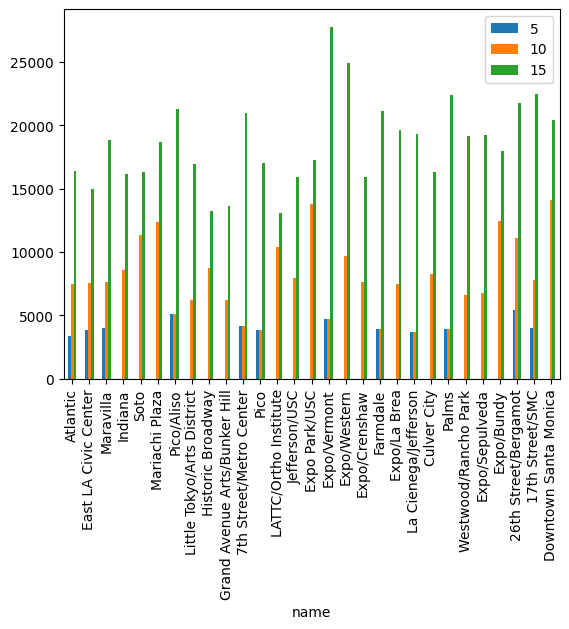
And here we can plot the number of people within 5, 10, and 15 minutes of each metro stop.

from pandas import DataFrame

times = [5, 10, 15]
data = []
for time in times:
    distance_to_time = lambda x: x / 1.35 < time * 60
    tdf = TripDataFrame(
        (distance_to_time(distance_dataframe) * 1).to_numpy()
        * zones_interpolated["Total Population + Worker Population"].to_numpy()[
            :, None
        ],
        index=zones_interpolated.index,
        columns=stops.name,
    ).astype(int)
    data.append(tdf.sum())

DataFrame(data=data, index=times, columns=distance_dataframe.columns).T.plot(kind="bar")

<Axes: xlabel='name'>

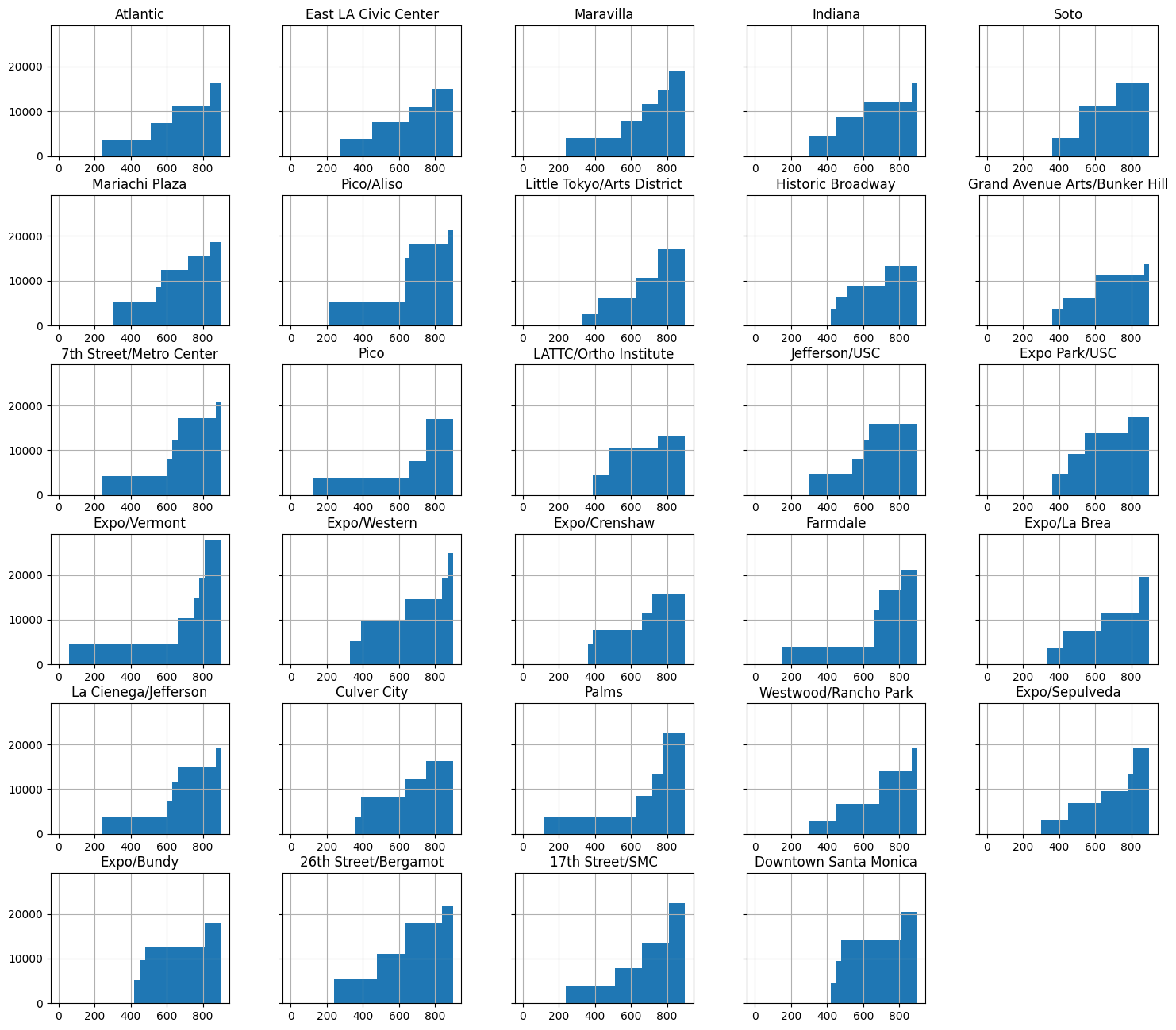
And here we can plot where people are within 15 minutes of a metro stop. This could be done much easier if we simply applied .buffer to each stop geometry.

And here we will plot the number of potential riders within 15 minutes of each stop.

from matplotlib import pyplot as plt

fig = plt.figure(figsize=(18, 16))
ax = fig.add_subplot(111)
(distance_dataframe / 1.35).hist(
    weights=zones_interpolated["Total Population + Worker Population"],
    range=(0, 900),
    bins=30,
    cumulative=True,
    sharey=True,
    ax=ax,
)
ax.set_ylabel("Population (cumulative)")
ax.set_xlabel("Time (seconds)")

/tmp/ipykernel_2518/1319192995.py:5: UserWarning: To output multiple subplots, the figure containing the passed axes is being cleared.
  (distance_dataframe / 1.35).hist(

Text(0.5, 0, 'Time (seconds)')

from mapclassify import Quantiles

zones_interpolated["Accessibility w/in 15 minutes"] = tdf.T.sum()
layer = SolidPolygonLayer.from_geopandas(zones_interpolated, opacity=0.1)
jc = Quantiles(zones_interpolated["Accessibility w/in 15 minutes"], k=10)
colors = []
for color in jc.yb:
    colors.append(Viridis_20.colors[color])
layer.get_fill_color = numpy.uint8(colors)
layers = [layer]

Map(layers=layers)

/home/docs/checkouts/readthedocs.org/user_builds/dpd/envs/latest/lib/python3.9/site-packages/lonboard/_geoarrow/ops/reproject.py:97: UserWarning: Input being reprojected to EPSG:4326 CRS
  warnings.warn("Input being reprojected to EPSG:4326 CRS")
/home/docs/checkouts/readthedocs.org/user_builds/dpd/envs/latest/lib/python3.9/site-packages/mapclassify/classifiers.py:1592: UserWarning: Not enough unique values in array to form 10 classes. Setting k to 2.
  self.bins = quantile(y, k=k)

Last, here are the Voronoi Polygons for the network. These show which is the closest stop for each polygon.

from shapely import voronoi_polygons, MultiPoint

stops = {}
for route in network.routes:
    for index, stop in network.routes[route].stops.iterrows():
        stops[stop["name"]] = stop["geometry"]

v = voronoi_polygons(MultiPoint(list(stops.values())), extend_to=los_angeles_county)

folium_map = folium.Map(location=(34, -118.3), zoom_start=11)
vs = GeoSeries(v.geoms, crs="EPSG:4326")
vs.intersection(los_angeles_county).explore(m=folium_map)
for route in network.routes:
    network.routes[route].stops.explore(m=folium_map)
folium_map

Make this Notebook Trusted to load map: File -> Trust Notebook