Four-step Transportation Model
This is an update of a blog post I wrote three years ago. I have since created classes to simplify the process of creating a four-step model. The two classes we will use are Zones and OriginDestinationDataFrame.
[1]:
import ipywidgets as widgets
from IPython.display import display
import matplotlib.pyplot as plt
import us

from dpd.modeling import Zones, OriginDestinationDataFrame
/usr/local/lib/python3.9/site-packages/geopandas/_compat.py:111: UserWarning: The Shapely GEOS version (3.9.1-CAPI-1.14.2) is incompatible with the GEOS version PyGEOS was compiled with (3.9.0-CAPI-1.16.2). Conversions between both will be slow.
  warnings.warn(
WARNING:param.main: pandas could not register all extension types imports failed with the following error: cannot import name 'ABCIndexClass' from 'pandas.core.dtypes.generic' (/usr/local/lib/python3.9/site-packages/pandas/core/dtypes/generic.py)
[2]:
YEAR = "2017"

state = widgets.Select(
    options=list(map(lambda x: x.name, us.STATES)), description="State", rows=10
)
display(state)
The Zones class defines our analysis zones for the four step model. It is based on a Geopandas GeoDataFrame so it includes a geometry column that maps each zone. The other important columns are Production and Attraction which include the production and attraction data for each zone and the index which is used by the OriginDestinationDataFrame. Zones can be automatically created from US Census data with the from_uscensus method. Otherwise you need to create a GeoDataFrame with the aforementioned columns.
[3]:
zones = Zones.from_uscensus(str(us.states.lookup(state.value).fips), YEAR)
/usr/local/lib/python3.9/site-packages/dpd/uscensus/get_uscensus_data.py:31: FutureWarning: Could not cast to int64, falling back to object. This behavior is deprecated. In a future version, when a dtype is passed to 'DataFrame', either all columns will be cast to that dtype, or a TypeError will be raised.
  dataframe = pandas.DataFrame(
[4]:
zones.head(1)
[4]:
| Name | Production | Attraction | state | county | tract | STATEFP | COUNTYFP | TRACTCE | NAME_y | ... | FUNCSTAT | ALAND | AWATER | INTPTLAT | INTPTLON | geometry | ProductionAttractionSum | Production Density | Attraction Density | ProductionAttractionSum Density | |
|---|---|---|---|---|---|---|---|---|---|---|---|---|---|---|---|---|---|---|---|---|---|
| GEOID | |||||||||||||||||||||
| 35049001002 | Census Tract 10.02, Santa Fe County, New Mexico | 3612 | 0 | 35 | 049 | 001002 | 35 | 049 | 001002 | 10.02 | ... | S | 2086269 | 0 | +35.6654818 | -105.9636628 | POLYGON ((-105.97726 35.66269, -105.97708 35.6... | 3612 | 1731.320362 | 0.0 | 1731.320362 |
1 rows × 22 columns
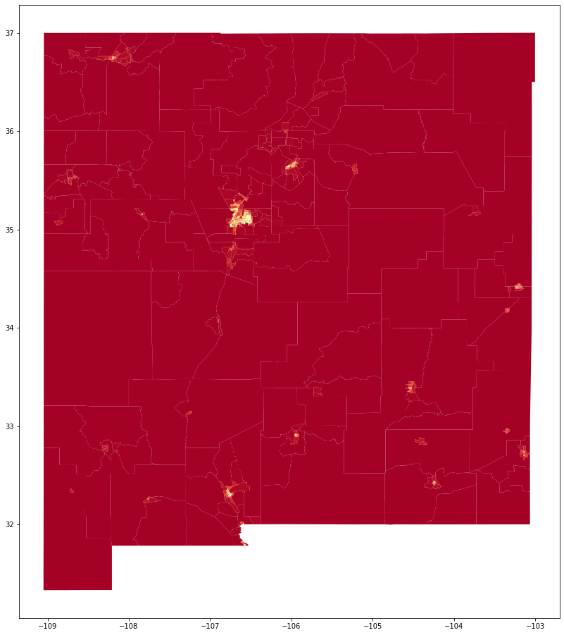
One of nice things about this being a GeoDataFrame is that you can easily plot it. In this case we can plot the “Production density” which is really just the population density. We can see each zone (big in rural areas, small in urban areas) and we can see the urban areas have higher densities. This is step one of our four-step model.
[5]:
zones["Production density"] = zones["Production"].map(int) / zones["ALAND"]
fig = plt.figure(figsize=(18, 16))
ax = fig.add_subplot(111)
zones.plot(column="Production density", cmap="RdYlGn", ax=ax)
[5]:
<AxesSubplot:>
Next we need to create a OriginDestinationDataFrame. We could compute this directly from our Zones object above, but we can also create this by downloading the US Census LODES data using the from_lodes method. This data is already organized as an origin-destination matrix. This is step two of the four-step model.
[6]:
od = TripDataFrame.from_lodes(us.states.lookup(state.value).abbr.lower(), YEAR)
/usr/local/lib/python3.9/site-packages/dpd/modeling/origin_destination_dataframe.py:41: DtypeWarning: Columns (28,29,31,37,38) have mixed types. Specify dtype option on import or set low_memory=False.
  xwalk = pandas.read_csv(download_lodes_xwalk(st))
[7]:
od
[7]:
| w_geocode | h_geocode | S000 | SA01 | SA02 | SA03 | SE01 | SE02 | SE03 | SI01 | SI02 | SI03 | createdate | ||
|---|---|---|---|---|---|---|---|---|---|---|---|---|---|---|
| trct_w | trct_h | |||||||||||||
| 35001000107 | 35001000107 | 6300180019282126 | 6300180019290148 | 22 | 0 | 9 | 13 | 7 | 8 | 7 | 2 | 0 | 20 | 363619980 |
| 35001000108 | 1050030003214025 | 1050030003244008 | 3 | 1 | 1 | 1 | 0 | 3 | 0 | 0 | 0 | 3 | 60603330 | |
| 35001000109 | 350010001071008 | 350010001091010 | 1 | 0 | 1 | 0 | 1 | 0 | 0 | 0 | 0 | 1 | 20201110 | |
| 35001000111 | 350010001071008 | 350010001112007 | 1 | 1 | 0 | 0 | 0 | 0 | 1 | 0 | 0 | 1 | 20201110 | |
| 35001000112 | 1750050005356019 | 1750050005607029 | 5 | 0 | 0 | 5 | 3 | 0 | 2 | 1 | 0 | 4 | 101005550 | |
| ... | ... | ... | ... | ... | ... | ... | ... | ... | ... | ... | ... | ... | ... | ... |
| 35061971400 | 35061970902 | 7012394280036520 | 7012394180421028 | 22 | 12 | 4 | 6 | 5 | 11 | 6 | 8 | 8 | 6 | 404022200 |
| 35061971000 | 17180365986092544 | 17180365790119452 | 62 | 15 | 38 | 9 | 4 | 40 | 18 | 13 | 38 | 11 | 989854390 | |
| 35061971100 | 4207436568023410 | 4207436532013085 | 13 | 3 | 8 | 2 | 1 | 6 | 6 | 2 | 8 | 3 | 242413320 | |
| 35061971300 | 3506197140017249 | 3506197130011257 | 11 | 3 | 7 | 1 | 2 | 6 | 3 | 1 | 2 | 8 | 202011100 | |
| 35061971400 | 16128506844079148 | 16128506844079080 | 66 | 16 | 35 | 15 | 14 | 27 | 25 | 13 | 23 | 30 | 929251060 |
88273 rows × 13 columns
Notice we use a multi-index instead of an index and column. This is because most zones do not have trips to other zones. We could unstack this dataframe to create a dataframe with the index as the origin and the columns as the destination. However, this creates many relationships (159,845 or 65% in this case) with no trips (NaN).
[8]:
od["S000"].unstack()
[8]:
| trct_h | 35001000107 | 35001000108 | 35001000109 | 35001000110 | 35001000111 | 35001000112 | 35001000113 | 35001000114 | 35001000115 | 35001000116 | ... | 35061970404 | 35061970405 | 35061970700 | 35061970800 | 35061970901 | 35061970902 | 35061971000 | 35061971100 | 35061971300 | 35061971400 |
|---|---|---|---|---|---|---|---|---|---|---|---|---|---|---|---|---|---|---|---|---|---|
| trct_w | |||||||||||||||||||||
| 35001000107 | 22.0 | 3.0 | 1.0 | NaN | 1.0 | 5.0 | 2.0 | 2.0 | 1.0 | 1.0 | ... | NaN | NaN | 2.0 | NaN | NaN | NaN | NaN | NaN | NaN | NaN |
| 35001000108 | 8.0 | 16.0 | 6.0 | 2.0 | 13.0 | 3.0 | 6.0 | 3.0 | 8.0 | 1.0 | ... | NaN | NaN | NaN | NaN | 3.0 | NaN | NaN | NaN | 1.0 | 2.0 |
| 35001000109 | 5.0 | 10.0 | 31.0 | 16.0 | 8.0 | 8.0 | 16.0 | 9.0 | 14.0 | 4.0 | ... | 4.0 | 1.0 | 1.0 | NaN | 2.0 | 1.0 | 3.0 | 2.0 | 1.0 | NaN |
| 35001000110 | 7.0 | 8.0 | 5.0 | 20.0 | 15.0 | 8.0 | 7.0 | 4.0 | 10.0 | 3.0 | ... | NaN | NaN | 1.0 | NaN | NaN | NaN | 1.0 | NaN | NaN | 4.0 |
| 35001000111 | 4.0 | 5.0 | 1.0 | 9.0 | 18.0 | 3.0 | 6.0 | 5.0 | 1.0 | 2.0 | ... | 2.0 | NaN | 1.0 | 2.0 | NaN | 4.0 | 1.0 | 1.0 | NaN | 2.0 |
| ... | ... | ... | ... | ... | ... | ... | ... | ... | ... | ... | ... | ... | ... | ... | ... | ... | ... | ... | ... | ... | ... |
| 35061970902 | NaN | NaN | NaN | NaN | NaN | NaN | NaN | NaN | NaN | NaN | ... | 3.0 | 3.0 | 4.0 | 4.0 | 5.0 | 5.0 | 2.0 | 3.0 | 2.0 | 1.0 |
| 35061971000 | NaN | NaN | NaN | 1.0 | NaN | 1.0 | NaN | 1.0 | NaN | NaN | ... | 19.0 | 6.0 | 30.0 | 48.0 | 22.0 | 5.0 | 56.0 | 9.0 | 12.0 | 9.0 |
| 35061971100 | NaN | NaN | NaN | NaN | NaN | NaN | NaN | NaN | NaN | NaN | ... | NaN | NaN | 4.0 | 11.0 | 10.0 | 3.0 | 7.0 | 8.0 | 3.0 | NaN |
| 35061971300 | NaN | NaN | NaN | NaN | NaN | NaN | NaN | NaN | NaN | NaN | ... | 1.0 | NaN | 14.0 | 10.0 | 23.0 | 8.0 | 9.0 | 8.0 | 13.0 | 1.0 |
| 35061971400 | 2.0 | 1.0 | 2.0 | 5.0 | 1.0 | 1.0 | 3.0 | 2.0 | 2.0 | 2.0 | ... | 115.0 | 67.0 | 59.0 | 49.0 | 54.0 | 22.0 | 62.0 | 13.0 | 11.0 | 66.0 |
496 rows × 499 columns
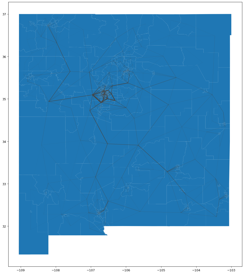
We are going to skip step three for now. That step will probably get its own notebook. In step four, we assign traffic to our transportation network. For this we need to create a network. We start by building a simple network based on our zones by reducing each zone to it’s centroid. We then connect the neighboring centroids.
[9]:
zones.build_graph()
/usr/local/lib/python3.9/site-packages/geopandas/geodataframe.py:199: UserWarning: Pandas doesn't allow columns to be created via a new attribute name - see https://pandas.pydata.org/pandas-docs/stable/indexing.html#attribute-access
  super().__setattr__(attr, val)
[9]:
<networkx.classes.graph.Graph at 0x130914ee0>
We can then assign our OriginDestinationDataFrame traffic to our Zones transportation network.
[10]:
od.route_assignment(zones)
[10]:
<networkx.classes.graph.Graph at 0x130914ee0>
And we can plot the final result. This looks about right at first glance. Please take a look at the underlying methods to see what is going on.
[11]:
fig = plt.figure(1, figsize=(18, 16), dpi=90)
ax = fig.add_subplot(111)
zones.visualize_route_assignment(ax=ax)
[12]:
zones.head()
[12]:
| Name | Production | Attraction | state | county | tract | STATEFP | COUNTYFP | TRACTCE | NAME_y | ... | INTPTLAT | INTPTLON | geometry | ProductionAttractionSum | Production Density | Attraction Density | ProductionAttractionSum Density | Production density | aea_centroid | centroid | |
|---|---|---|---|---|---|---|---|---|---|---|---|---|---|---|---|---|---|---|---|---|---|
| GEOID | |||||||||||||||||||||
| 35049001002 | Census Tract 10.02, Santa Fe County, New Mexico | 3612 | 0 | 35 | 049 | 001002 | 35 | 049 | 001002 | 10.02 | ... | +35.6654818 | -105.9636628 | POLYGON ((-105.97726 35.66269, -105.97708 35.6... | 3612 | 1731.320362 | 0.0 | 1731.320362 | 1.731320e-03 | POINT (35.665 -105.964) | POINT (35.665 -105.964) |
| 35049010400 | Census Tract 104, Santa Fe County, New Mexico | 3423 | 0 | 35 | 049 | 010400 | 35 | 049 | 010400 | 104 | ... | +35.6547921 | -105.8796126 | POLYGON ((-105.93988 35.65773, -105.93959 35.6... | 3423 | 81.175154 | 0.0 | 81.175154 | 8.117515e-05 | POINT (35.654 -105.892) | POINT (35.654 -105.892) |
| 35049001103 | Census Tract 11.03, Santa Fe County, New Mexico | 1731 | 0 | 35 | 049 | 001103 | 35 | 049 | 001103 | 11.03 | ... | +35.6560820 | -105.9712060 | POLYGON ((-105.98489 35.65625, -105.98488 35.6... | 1731 | 777.802741 | 0.0 | 777.802741 | 7.778027e-04 | POINT (35.656 -105.971) | POINT (35.656 -105.971) |
| 35049000600 | Census Tract 6, Santa Fe County, New Mexico | 2030 | 0 | 35 | 049 | 000600 | 35 | 049 | 000600 | 6 | ... | +35.6758514 | -105.9446226 | POLYGON ((-105.95818 35.67497, -105.95643 35.6... | 2030 | 1244.532182 | 0.0 | 1244.532182 | 1.244532e-03 | POINT (35.676 -105.945) | POINT (35.676 -105.945) |
| 35059950200 | Census Tract 9502, Union County, New Mexico | 4216 | 0 | 35 | 059 | 950200 | 35 | 059 | 950200 | 9502 | ... | +36.4880853 | -103.4757229 | POLYGON ((-104.00934 36.69766, -104.00823 36.6... | 4216 | 0.425692 | 0.0 | 0.425692 | 4.256922e-07 | POINT (36.482 -103.471) | POINT (36.482 -103.471) |
5 rows × 25 columns
[ ]: